Only Math You Need Before Coding your Algo Trading Strategy
You do not need advanced calculus to begin algorithmic trading. You do need a small, disciplined toolkit: measure returns consistently, describe uncertainty with probability, estimate expected outcomes, understand dispersion, respect sampling error and follow compounding. These ideas make a trading hypothesis precise. They do not create an edge, predict the next trade or guarantee a profit.
The examples in this article are deliberately small and synthetic. They explain the arithmetic; they are not trading results.
Start with the question, not the formula
When people hear “maths for algorithmic trading”, they often picture calculus, differential equations or a wall of statistical notation. That is the wrong starting point. Before you write a line of Python, you need to answer a much simpler question: what exactly will your rule measure, and what would count as evidence that it is useful?
A trading rule turns information, such as price, volume, time or an order state, into a decision. The decision then produces one of several possible outcomes. Good maths helps you describe that chain without hiding assumptions:
- What was the observation: a price change, a filled trade, a return or a profit-and-loss result?
- What information was available when the decision was made?
- How often did each outcome occur?
- How large were the wins and losses after realistic costs?
- How much does the result vary, and how much information supports it?
That is enough to begin thinking like a quantitative researcher. The six ideas below provide the vocabulary.
Returns: measure the change before you interpret it
A return is a change relative to a stated starting value. For a price series, the simple return from one observation to the next is:
rₜ = (Pₜ / Pₜ₋₁) − 1
If a price moves from ₹100 to ₹103, the simple return is 3%. The arithmetic is easy; the definition is where many backtests go wrong. A 3% close-to-close return, a 3% move between five-minute bars and a 3% fill-to-fill return are not interchangeable. Each describes a different observation.
Log returns use the natural logarithm:
ℓₜ = ln(Pₜ / Pₜ₋₁)
Their useful property is that consecutive log returns add, which can make some modelling tasks more convenient. Simple returns are usually easier to explain and report. Either way, state the price basis, timestamp and interval; never mix simple and log returns silently.
The same discipline applies to Indian-market data. Corporate actions, missing prices, time zones and instrument identity can change the meaning of a return. If you are not sure whether a number represents a close, a tradable fill or an adjusted price, read the clean NSE data pipeline and data-quality checks before drawing a conclusion.
Probability: ask what happens after the condition
Probability gives a strategy a way to talk about uncertainty. It does not mean that the code knows the future. It means that, under a defined information set, different outcomes have different observed or assumed frequencies.
An unconditional question asks for a base rate: how often did the market rise across the full sample? A conditional question is narrower: how often did it rise after condition B occurred?
P(A | B) = P(A ∩ B) / P(B)
The denominator matters. Suppose a signal appeared 12 times and 9 of those observations were followed by a gain. It is accurate to say that 9 of 12, or 75%, were gains in that sample. It is not accurate to present “75% success” without showing how often the signal appeared, what the baseline was and how the observations were selected.
A conditional result also needs a clearly defined event, universe, timeframe and sampling method. Did “after the signal” mean the next close, the next five-minute bar or the next executable fill? Did the universe include every eligible security at the time, or only today’s survivors? Before calculating, make sure the market sessions, lots and settlement conventions match the question you are asking.
Probability is most useful when it keeps you honest about the denominator. A rare signal can produce a striking percentage that becomes ordinary or disappears when more observations arrive.
Expected value: why a 60% win rate can still lose
Expected value is a probability-weighted average of possible outcomes. The NIST Tutorial for Metrologists describes expectation as the weighted mean of a random variable’s distribution (1). It summarises the centre of the distribution; it does not predict the next observation.
E[X] = Σ pᵢxᵢ
For a trading rule, a useful expectancy calculation combines the chance of a win, the average win, the chance of a loss, the average loss and the expected cost of trading. If wins and losses are measured in the same risk unit, R, a simple net form is:
E[R_net] = p × W − (1 − p) × L − E[c]
Here, p is the win probability, W is the average win in R, L is the positive magnitude of the average loss in R, and E[c] is the expected cost per trade, also in R. Every term must use the same unit. If costs are kept in rupees, convert the payoff terms to rupees as well. Spread, slippage, brokerage, exchange charges and taxes can all reduce the result; use the current Indian trading-cost guide for live fee assumptions.
The payoff matters as much as the win rate
Consider three entirely synthetic trade distributions:
| Case | Win rate | Average win | Average loss | Gross expectancy | Net after 0.10R cost |
| A | 45% | +2.0R | −1.0R | +0.35R | +0.25R |
| B | 60% | +0.8R | −1.5R | −0.12R | −0.22R |
| C | 35% | +3.0R | −1.0R | +0.40R | +0.30R |
Case A wins less than half the time but remains positive under the stated assumptions because its winners are twice the size of its average loss. Case B wins more often yet loses because its losses are too large. Case C makes the same point more strongly. The examples do not estimate what a real strategy can achieve; they show why a win rate cannot stand in for expectancy.
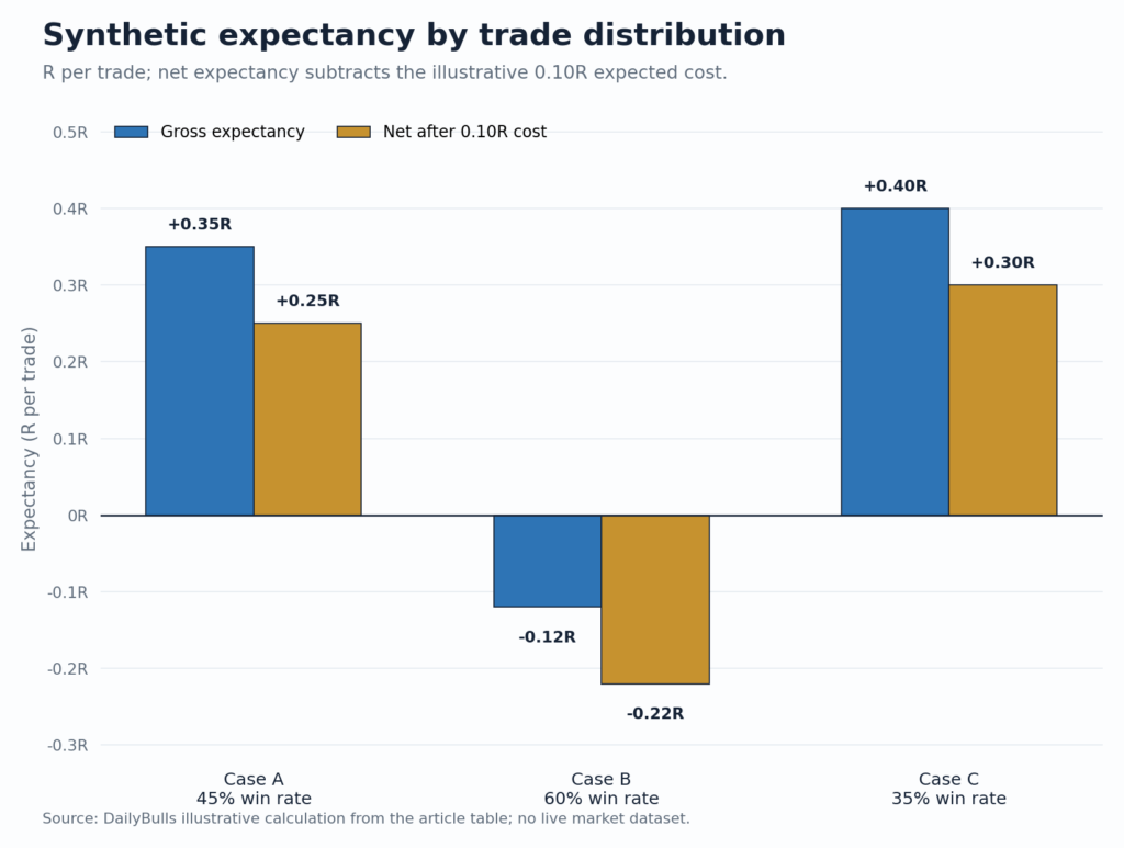
Synthetic gross and net expectancy by trade distribution. Net expectancy subtracts an illustrative 0.10R cost; no case is a historical result. Source: DailyBulls illustrative calculation.
For a deeper vocabulary around profit factor, drawdown and average R, the backtest-metrics guide expands the measurement framework. Expectancy is the bridge between a rule’s outcomes and the question “does the payoff still make sense after costs?”
Dispersion and sample size: how much trust does the average deserve?
Two strategies can have the same average return while behaving very differently. Dispersion describes how widely outcomes vary around their average. Variance is the expected squared distance from the mean, and standard deviation is the positive square root of variance. NIST gives the construction as (1):
Var(X) = E[(X − E[X])²]
SD(X) = √Var(X)
For a finite sample, the sample mean is x̄ = (1/n)Σxᵢ, and the usual sample variance uses n − 1 in the denominator. The denominator is a reminder that a backtest is a sample, not the entire distribution of future outcomes.
Dispersion is not the same as drawdown, tail loss, liquidity risk or an order rejection. A strategy with a high average and wide variation may be harder to interpret than one with a smaller but more stable average. The right measure depends on the decision you are making; Backtest Metrics That Matter covers the wider metric set.
Sample size adds another layer of caution:
- A 9-for-12 result is not equivalent to 900-for-1,200, even though both show 75%.
- Overlapping trades or repeated signals during one market episode can make the raw count look larger than the independent information available.
- A sample that ends before a difficult market regime can omit the outcomes that matter most.
- Testing many variants and reporting only the one that looked best creates a selection problem, even if every calculation was arithmetically correct.
Maths cannot remove these problems. It can force you to show the denominator, define the event, compare a baseline and record the conditions under which the calculation was made. Chronological out-of-sample testing, walk-forward analysis and Monte Carlo methods are the next layer once this vocabulary is clear.
Compounding: the order of returns changes capital
Capital compounds by multiplying growth factors. Start with one unit. A gain of 10% followed by a loss of 10% gives:
1 × 1.10 × 0.90 = 0.99
The sequence ends 1% below the starting value even though the arithmetic average of +10% and −10% is zero. The Investor.gov explanation of compound interest uses the same basic idea: returns are applied to a changing base (2). In trading, that base can shrink as well as grow, so compounding is not a promise of wealth.
This is why a backtest should report more than an average trade. The return convention, exposure, order of outcomes, withdrawals and changing position size can all affect the path of capital. A sequence of small losses followed by a recovery is not equivalent to the same numbers in the opposite order. Position sizing and loss limits are separate decisions; they should not be smuggled into a simple compounding example.
An edge is a hypothesis, not a feeling
An edge is not a synonym for a high win rate, a sophisticated indicator or a good-looking equity curve. For research, it is a testable difference between a rule and a clearly defined baseline after realistic costs, with a reason that could explain why the difference exists.
A useful pre-coding statement might be:
When condition B is present, the next five-minute return distribution will differ from the unconditional distribution by at least X, after a stated cost assumption.
That sentence is not a recommendation. It is a specification that can be rejected. It tells you what information is used, what outcome is measured, which baseline is being compared, how long the measurement lasts and what result would make the idea fail.
Before opening a notebook, write down:
- the observation: price, return, fill, P&L or risk-unit outcome;
- the timestamp and timezone;
- the universe and eligibility rule;
- the unconditional baseline;
- the conditional event and its denominator;
- the average win, average loss and expected cost;
- the dispersion and dependence you will check;
- the result that would make you abandon the idea before optimisation.
This is the point at which maths becomes useful to a researcher. It turns “I think this pattern works” into a claim that data can challenge.
What this maths can and cannot do
These ideas can help you define returns, compare payoff with win rate, describe dispersion, expose small samples and write a falsifiable research question. They cannot predict the next trade with certainty, turn a historical average into a guaranteed edge, make biased data reliable or choose a personal position size for you.
That boundary is important. A formula can be correct while the dataset is incomplete, the fills are unrealistic or the hypothesis was chosen after looking at the answer. Quantitative work is not about making uncertainty disappear; it is about making uncertainty visible.
The practical next step
You now have enough maths to begin coding: not because the formulas promise a result, but because they tell you what your code must measure. Set up a reproducible Python environment, calculate a few returns by hand, and make your first notebook print the denominator, payoff, costs and dispersion alongside any headline result.
Start with Python Setup for Trading (Windows), then move to a clean data pipeline and a backtest whose assumptions you can inspect. The useful habit is simple: define the number before you trust it.
Sources
The numerical cases in this article are synthetic and labelled; no live market dataset or performance claim is used. Any future India-specific example should state its universe, period, frequency, price basis, costs and exclusions.
Share this insight
Spread the Alpha
Related Articles
More ideas that align with your trading playbook.
Data QA before Algo Trading backtesting: why your dataset can mislead you
A backtest can be wrong even when the file opens, the candles look plausible and the code runs without an exception. Current-only…
pandas for Algo Trading Data: A Practical Crash Course for Candle Data
Pandas becomes useful for trading research when you make time, price fields and table grain explicit. Sort each instrument’s timestamps, define the…
Building a Clean NSE Data Pipeline for Algo Trading: From Bhavcopy to Research-Ready Candles
Building a clean NSE data pipeline means more than download a file. It preserves the original input, records where each row came…
 DailyBulls (Arthashilpi Ventures) is a D-U-N-S verified company.