Testing the 20/50 SMA Crossover Algo Strategy on Nifty 50
When you first learn about moving average crossovers, the concept seems almost too simple. Two lines on a chart. They cross. You buy. They diverge. You sell. Yet here’s the thing, simplicity is exactly why it’s worth testing. We backtested the 20 & 50 SMA Crossover strategy for algorithmic traders on over a decade of Nifty 50’s data, to see what really happens in theory. Is this classic book strategy actually useful in algo trading, or you’d end up in red?
What we found was equal parts illuminating and frustrating. And educational. This article walks through everything we discovered: what worked, what failed spectacularly, and why the difference between the two came down to something most traders overlook completely.
Understanding the 20 and 50 Simple Moving Average Strategy
How It Works
The logic is straightforward enough that any trader can implement it tomorrow in python. We also attached the codes at the end of this article so you can replicate the strategy. We calculate two simple moving averages on Nifty 50’s daily closing prices. One tracks the past 20 days. The other looks back 50 days, basically these are 20 and 50 period simple moving averages.
Here’s the signal: When the 20-day average crosses above the 50-day average, something shifts. The market appears to be transitioning from a downtrend (or sideways movement) into actual upward momentum. That’s our entry cue.
But we don’t jump in immediately. Instead, we wait for the next trading day and enter at the opening price for confirmation.
Risk Management Approach
Every trade taken in the 20/50 SMA strategy follows a fixed 1:2 RR ratio. Stop-loss is at 1% below entry. We target profit of 2% above entry. That means you’re risking 1 rupee to potentially make 2. In theory, you could win just one out of three trades and still break even (considering your winners and losers maintain this exact ratio)
Sounds reasonable on paper. Let’s see what actually happened.
Exit Logic
The system checks for exits in a specific order each trading day:
1. Gap Opens : If the market opens below the SL, we exit at that open price. If it opens above the profit target, we take the win immediately.
2. Intraday Hits: If during the day the low touches the stop, we exit. If the high reaches the profit target, we book.
3. Signal Reversal: If the 20-day average falls back below the 50-day average while we are in the trade, we exit at the close.
Part 1: Fixed Stops Loss Strategy with SMA 20/50 Crossover
The Problem With Tight Stops
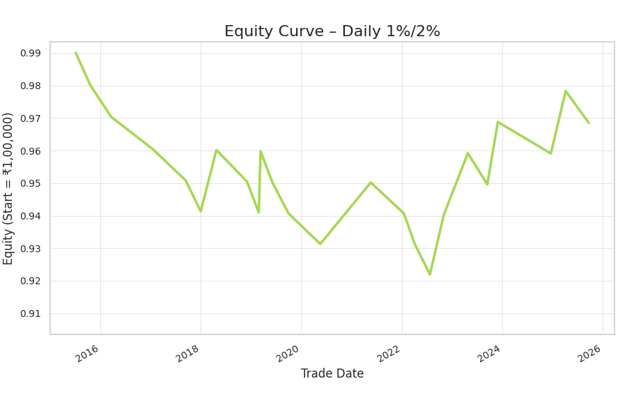
Between 2015 and October 2025, the strategy generated 24 distinct trading signals. In the last 10 years, the strategy generated 24 signals. So this 20 and 50 MA strategy is definitely not for someone who is looking for a more aggressive number of entries. I have shared the results below.
| Metric | Value |
|---|---|
| Win Rate | 29% |
| Total Return | -3.15% |
| Maximum Drawdown | -6.87% |
| Starting Capital | ₹1,00,000 |
| Ending Capital | ₹96,850 |
| Duration | 10 Years |
The average payoff per trade was -0.12R. Winners weren’t large enough to offset our losers. That’s negative expectancy. The Algo strategy of 20 and 50 moving average did not prove to be profitable in the past decade.
Why It Failed
The 1% stop proved too tight for how Nifty 50 actually moves. Normal market volatility would trigger the stop, and then the market would reverse and move exactly where we wanted it to be. This happened repeatedly. Most trades hit the stop within days. Sometimes the same day we entered.
Here’s every single trade over the 10-year period.
| Entry Date | Entry Price | Exit Date | Exit Price | P&L | Return |
|---|---|---|---|---|---|
| 2015-07-08 | 8439.2 | 2015-07-08 | 8354.81 | -84.39 | -1.0% |
| 2015-10-21 | 8258.35 | 2015-10-28 | 8175.77 | -82.58 | -1.0% |
| 2016-03-22 | 7695.55 | 2016-03-28 | 7618.59 | -76.96 | -1.0% |
| 2017-01-17 | 8415.05 | 2017-01-23 | 8329.6 | -85.45 | -1.02% |
| 2017-09-13 | 10099.2 | 2017-09-22 | 9998.26 | -100.99 | -1.0% |
| 2018-01-01 | 10531.7 | 2018-01-01 | 10426.4 | -105.32 | -1.0% |
| 2018-04-25 | 10612.4 | 2018-05-14 | 10824.6 | 212.25 | 2.0% |
| 2018-12-03 | 10930.7 | 2018-12-05 | 10820.5 | -110.25 | -1.01% |
| 2019-02-27 | 10881.2 | 2019-02-27 | 10772.4 | -108.81 | -1.0% |
| 2019-03-12 | 11231.4 | 2019-03-15 | 11456 | 224.63 | 2.0% |
| 2019-06-06 | 12039.8 | 2019-06-06 | 11919.4 | -120.4 | -1.0% |
| 2019-10-01 | 11515.4 | 2019-10-01 | 11400.2 | -115.15 | -1.0% |
| 2020-05-19 | 8961.7 | 2020-05-19 | 8872.08 | -89.62 | -1.0% |
| 2021-05-21 | 14987.8 | 2021-05-25 | 15291.8 | 303.95 | 2.03% |
| 2022-01-17 | 18235.7 | 2022-01-19 | 18053.3 | -182.36 | -1.0% |
| 2022-04-06 | 17842.8 | 2022-04-07 | 17664.3 | -178.43 | -1.0% |
| 2022-07-25 | 16662.5 | 2022-07-26 | 16495.9 | -166.63 | -1.0% |
| 2022-11-04 | 18053.4 | 2022-11-15 | 18414.5 | 361.07 | 2.0% |
| 2023-04-27 | 17813.1 | 2023-05-02 | 18169.4 | 356.26 | 2.0% |
| 2023-09-15 | 20156.5 | 2023-09-20 | 19954.9 | -201.56 | -1.0% |
| 2023-12-01 | 20194.1 | 2023-12-04 | 20602 | 407.85 | 2.02% |
| 2024-12-20 | 23960.7 | 2024-12-20 | 23721.1 | -239.61 | -1.0% |
| 2025-04-07 | 21758.4 | 2025-04-07 | 22193.6 | 435.17 | 2.0% |
| 2025-09-22 | 25238.1 | 2025-09-25 | 24985.7 | -252.38 | -1.0% |
Notice the pattern from this data. Stops hit. 1% losses. Again and again. Meanwhile, the few winning trades of 2% weren’t big enough to compensate for all those 1% losses.
Key Learning
Here’s what many traders learn the hard way: tight stops that sound conservative actually amplify losses. They force you out of trades that would’ve been profitable if you’d place dynamic stop losses instead of fixed 1%.
Part 2: ATR-Based Stops 20&50 SMA Crossover Algo Strategy
We couldn’t ignore what the data was showing. Fixed stops were killing the gains in our strategy. So we tried something different: ATR-based trailing stops.
ATR stands for Average True Range. It’s basically a volatility measure that adapts to current conditions. When volatility is low, ATR is small, so stops are tighter. When volatility spikes, ATR gets bigger so stops widen.
The stop adapts to what the market is actually doing instead of forcing the same rigid rule onto every situation.
We set the initial stop at 1.5 times the ATR value below entry. Then, each day, we recalculate the ATR and trail the stop upward.
Dramatic Performance Improvement
| Metric | Value |
|---|---|
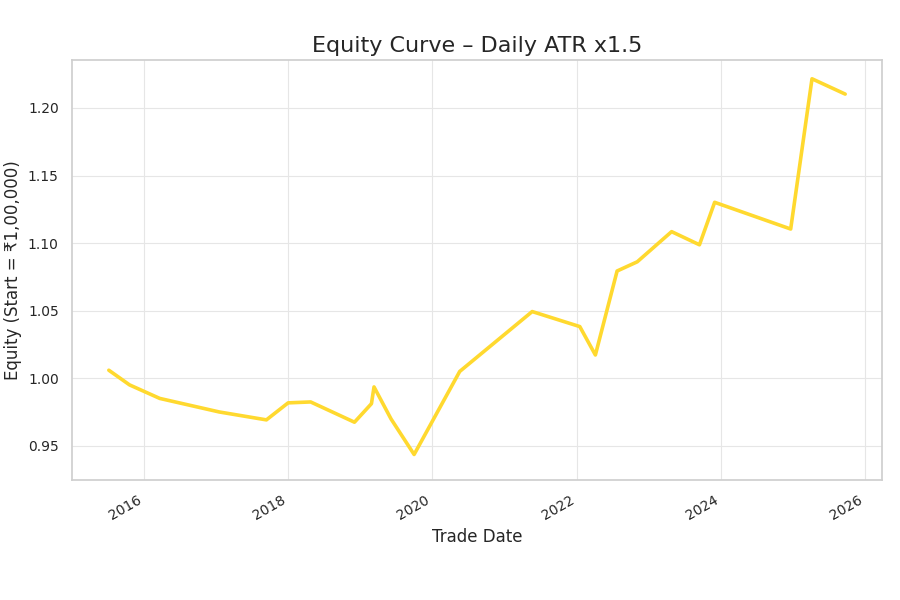
| Trades | 24 |
| Win Rate | 50% (12/24) |
| Total Return | +21.03% |
| Maximum Drawdown | -6.19% |
| Starting Capital | ₹1,00,000 |
| Ending Capital | ₹1,21,030 |
| Duration | 10 Years |
That’s a 24% difference. The entry signal didn’t change. The exit strategy did. And that’s the entire difference.
This is the core insight worth remembering: exit strategy matters more than entry strategy.
Why It Worked Better
With ATR stops, something different happened. Winning trades stayed open. Weeks. Sometimes months. The market had room to actually develop the trend you’d identified.
Look at these results:
| Period | Return (%) | Duration (Days) |
|---|---|---|
| April–May 2025 | 10.01% | 32 |
| July–August 2022 | 6.10% | 28 |
| June 2021 | 4.41% | 27 |
| May 2023 | 2.05% | 20 |
| May 2019 | 1.42% | 9 |
| December 2023 | 2.86% | 12 |
Complete Daily ATR Trade Ledger
Here’s the complete picture of what happens when you let volatility guide your stops instead of forcing a fixed percentage:
| Entry Date | Entry Price | Exit Date | Exit Price | P&L | Return | Days |
|---|---|---|---|---|---|---|
| 2015-07-08 | 8439.2 | 2015-07-27 | 8490.2 | 51 | 0.6% | 19 |
| 2015-10-21 | 8258.35 | 2015-10-28 | 8169.25 | -89.1 | -1.08% | 7 |
| 2016-03-22 | 7695.55 | 2016-04-05 | 7618.17 | -77.38 | -1.01% | 14 |
| 2017-01-17 | 8415.05 | 2017-01-23 | 8329.6 | -85.45 | -1.02% | 6 |
| 2017-09-13 | 10099.2 | 2017-09-22 | 10038.6 | -60.65 | -0.6% | 9 |
| 2018-01-01 | 10531.7 | 2018-01-17 | 10668.4 | 136.7 | 1.3% | 16 |
| 2018-04-25 | 10612.4 | 2018-05-04 | 10619.8 | 7.36 | 0.07% | 9 |
| 2018-12-03 | 10930.7 | 2018-12-05 | 10763.9 | -166.79 | -1.53% | 2 |
| 2019-02-27 | 10881.2 | 2019-03-08 | 11035.4 | 154.2 | 1.42% | 9 |
| 2019-03-12 | 11231.4 | 2019-03-25 | 11373.1 | 141.79 | 1.26% | 13 |
| 2019-06-06 | 12039.8 | 2019-06-17 | 11753.4 | -286.41 | -2.38% | 11 |
| 2019-10-01 | 11515.4 | 2019-10-04 | 11202.8 | -312.57 | -2.71% | 3 |
| 2020-05-19 | 8961.7 | 2020-06-12 | 9544.95 | 583.25 | 6.51% | 24 |
| 2021-05-21 | 14987.8 | 2021-06-17 | 15648.3 | 660.5 | 4.41% | 27 |
| 2022-01-17 | 18235.7 | 2022-01-19 | 18042.5 | -193.14 | -1.06% | 2 |
| 2022-04-06 | 17842.8 | 2022-04-12 | 17482 | -360.79 | -2.02% | 6 |
| 2022-07-25 | 16662.5 | 2022-08-22 | 17679.7 | 1017.17 | 6.1% | 28 |
| 2022-11-04 | 18053.4 | 2022-11-21 | 18167.2 | 113.82 | 0.63% | 17 |
| 2023-04-27 | 17813.1 | 2023-05-17 | 18179 | 365.88 | 2.05% | 20 |
| 2023-09-15 | 20156.5 | 2023-09-20 | 19979.7 | -176.78 | -0.88% | 5 |
| 2023-12-01 | 20194.1 | 2023-12-13 | 20771.5 | 577.4 | 2.86% | 12 |
| 2024-12-20 | 23960.7 | 2024-12-20 | 23541.8 | -418.89 | -1.75% | 0 |
| 2025-04-07 | 21758.4 | 2025-05-09 | 23935.8 | 2177.35 | 10.01% | 32 |
| 2025-09-22 | 25238.1 | 2025-09-25 | 25004.3 | -233.82 | -0.93% | 3 |
Part 3: Testing the 20 and 50 MA Strategy on Faster Timeframes
Intraday Strategy Testing
After seeing what worked on daily charts, the natural question was: would it work even better on faster timeframes? More trades per month. More opportunities. Right?
We tested 5-minute and 15-minute charts using recent data from August through October 2025. The results taught us something important about how market structure changes at different speeds.
5-Minute Charts: Speed vs. Noise
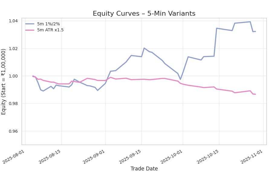
On 5-minute bars, we generated 46 trades across a two-month period.
With the fixed 1:2 R:R approach, we achieved 41.3% win rate with +3.22% return.
The ATR approach: 28.3% win rate, -1.33% return.
Wait, that’s the opposite of what we saw on daily charts. Why?
On a 5-minute timeframe, the market is incredibly noisy relative to actual trends. The 1% fixed stop, too tight for daily charts, actually works here. The ATR trailing stop becomes too aggressive. It closes winning positions before the real move happens because ATR on 5-minute bars reacts to every small price fluctuation.
Speed doesn’t always equal better.
5-Minute Fixed Stop Trades – Complete Ledger
| Entry Date | Entry Price | Exit Date | Exit Price | P&L | Return |
|---|---|---|---|---|---|
| 2025-08-04 | 24626 | 2025-08-05 | 24614.5 | -11.4 | -0.05% |
| 2025-08-05 | 24624.5 | 2025-08-05 | 24615.8 | -8.8 | -0.04% |
| 2025-08-06 | 24650.5 | 2025-08-06 | 24564.6 | -85.95 | -0.35% |
| 2025-08-06 | 24617 | 2025-08-06 | 24580.8 | -36.2 | -0.15% |
| 2025-08-07 | 24534.3 | 2025-08-08 | 24427.2 | -107.2 | -0.44% |
| 2025-08-08 | 24424.8 | 2025-08-08 | 24403.4 | -21.35 | -0.09% |
| 2025-08-11 | 24462.2 | 2025-08-12 | 24546 | 83.8 | 0.34% |
| 2025-08-12 | 24575.5 | 2025-08-12 | 24531.8 | -43.6 | -0.18% |
| 2025-08-13 | 24582.3 | 2025-08-14 | 24649.1 | 66.75 | 0.27% |
| 2025-08-14 | 24633.4 | 2025-08-14 | 24629.2 | -4.15 | -0.02% |
| 2025-08-14 | 24657.8 | 2025-08-14 | 24642 | -15.85 | -0.06% |
| 2025-08-18 | 24945 | 2025-08-18 | 24930 | -15.1 | -0.06% |
| 2025-08-19 | 24935.5 | 2025-08-19 | 24975.1 | 39.6 | 0.16% |
| 2025-08-20 | 24997.2 | 2025-08-21 | 25100 | 102.8 | 0.41% |
| 2025-08-22 | 24930.5 | 2025-08-22 | 24878.5 | -52 | -0.21% |
| 2025-08-25 | 24914.3 | 2025-08-26 | 24850.5 | -63.75 | -0.26% |
| 2025-08-26 | 24806 | 2025-08-26 | 24800.5 | -5.55 | -0.02% |
| 2025-08-28 | 24584.5 | 2025-08-28 | 24557.9 | -26.6 | -0.11% |
| 2025-08-29 | 24563.4 | 2025-08-29 | 24508 | -55.35 | -0.23% |
| 2025-09-01 | 24528.6 | 2025-09-02 | 24655 | 126.45 | 0.52% |
| 2025-09-03 | 24571.2 | 2025-09-04 | 24788.7 | 217.55 | 0.89% |
| 2025-09-05 | 24757.5 | 2025-09-08 | 24768.8 | 11.3 | 0.05% |
| 2025-09-09 | 24818.5 | 2025-09-10 | 24973 | 154.5 | 0.62% |
| 2025-09-11 | 24984.7 | 2025-09-12 | 25101.8 | 117.2 | 0.47% |
| 2025-09-15 | 25091.4 | 2025-09-15 | 25069.9 | -21.5 | -0.09% |
| 2025-09-16 | 25151.8 | 2025-09-17 | 25307.3 | 155.5 | 0.62% |
| 2025-09-18 | 25424.8 | 2025-09-18 | 25359.3 | -65.45 | -0.26% |
| 2025-09-19 | 25317.9 | 2025-09-19 | 25324.5 | 6.55 | 0.03% |
| 2025-09-19 | 25342.3 | 2025-09-22 | 25305.1 | -37.25 | -0.15% |
| 2025-09-23 | 25196.5 | 2025-09-24 | 25069.1 | -127.45 | -0.51% |
| 2025-09-24 | 25115.1 | 2025-09-24 | 25058.4 | -56.7 | -0.23% |
| 2025-09-29 | 24785.8 | 2025-09-29 | 24640.5 | -145.25 | -0.59% |
| 2025-09-29 | 24727.1 | 2025-09-30 | 24665.7 | -61.45 | -0.25% |
| 2025-09-30 | 24677 | 2025-09-30 | 24601.4 | -75.65 | -0.31% |
| 2025-10-01 | 24664.8 | 2025-10-03 | 24791 | 126.2 | 0.51% |
| 2025-10-03 | 24821.2 | 2025-10-07 | 25100.8 | 279.6 | 1.13% |
| 2025-10-08 | 25116.2 | 2025-10-09 | 25059 | -57.3 | -0.23% |
| 2025-10-09 | 25152.8 | 2025-10-13 | 25213.8 | 60.95 | 0.24% |
| 2025-10-13 | 25184.8 | 2025-10-14 | 25192.3 | 7.45 | 0.03% |
| 2025-10-14 | 25173.6 | 2025-10-17 | 25677.1 | 503.47 | 2.0% |
| 2025-10-20 | 25860 | 2025-10-20 | 25817.3 | -42.6 | -0.16% |
| 2025-10-21 | 25886.5 | 2025-10-23 | 26020.8 | 134.25 | 0.52% |
| 2025-10-27 | 25921.7 | 2025-10-27 | 25947.8 | 26.05 | 0.1% |
| 2025-10-28 | 26028.7 | 2025-10-28 | 25880.8 | -147.85 | -0.57% |
| 2025-10-28 | 25879 | 2025-10-28 | 25817.8 | -61.2 | -0.24% |
| 2025-10-29 | 26010.8 | 2025-10-29 | 26043.5 | 32.8 | 0.13% |
Notice the pattern here too. Most trades are tiny. Very few reach the 2% target. Only one trade (October 14) actually hit the full 2% target. The rest are small gains and small losses, whipsawed by constant noise.
5-Minute ATR Trailing Stop Trades – Complete Ledger
| Entry Date | Entry Price | Exit Date | Exit Price | P&L | Return |
|---|---|---|---|---|---|
| 2025-08-04 | 24626 | 2025-08-04 | 24625.5 | -0.4 | -0.0% |
| 2025-08-05 | 24624.5 | 2025-08-05 | 24601.8 | -22.76 | -0.09% |
| 2025-08-06 | 24650.5 | 2025-08-06 | 24617.3 | -33.26 | -0.13% |
| 2025-08-06 | 24617 | 2025-08-06 | 24606.2 | -10.82 | -0.04% |
| 2025-08-07 | 24534.3 | 2025-08-08 | 24544.2 | 9.9 | 0.04% |
| 2025-08-08 | 24424.8 | 2025-08-08 | 24400.8 | -23.91 | -0.1% |
| 2025-08-11 | 24462.2 | 2025-08-11 | 24432.3 | -29.99 | -0.12% |
| 2025-08-12 | 24575.5 | 2025-08-12 | 24574.7 | -0.79 | -0.0% |
| 2025-08-13 | 24582.3 | 2025-08-13 | 24565.3 | -17.09 | -0.07% |
| 2025-08-14 | 24633.4 | 2025-08-14 | 24630.9 | -2.52 | -0.01% |
| 2025-08-14 | 24657.8 | 2025-08-14 | 24632.8 | -25.03 | -0.1% |
| 2025-08-18 | 24945 | 2025-08-18 | 24959.5 | 14.47 | 0.06% |
| 2025-08-19 | 24935.5 | 2025-08-19 | 24984.2 | 48.7 | 0.2% |
| 2025-08-20 | 24997.2 | 2025-08-20 | 24991.2 | -5.99 | -0.02% |
| 2025-08-22 | 24930.5 | 2025-08-22 | 24914.7 | -15.76 | -0.06% |
| 2025-08-25 | 24914.3 | 2025-08-25 | 24986.6 | 72.34 | 0.29% |
| 2025-08-26 | 24806 | 2025-08-26 | 24800.5 | -5.55 | -0.02% |
| 2025-08-28 | 24584.5 | 2025-08-28 | 24569.5 | -15 | -0.06% |
| 2025-08-29 | 24563.4 | 2025-08-29 | 24546.9 | -16.46 | -0.07% |
| 2025-09-01 | 24528.6 | 2025-09-01 | 24527.4 | -1.18 | -0.0% |
| 2025-09-03 | 24571.2 | 2025-09-03 | 24628.3 | 57.12 | 0.23% |
| 2025-09-05 | 24757.5 | 2025-09-05 | 24726.6 | -30.89 | -0.12% |
| 2025-09-09 | 24818.5 | 2025-09-09 | 24833.5 | 15.01 | 0.06% |
| 2025-09-11 | 24984.7 | 2025-09-11 | 24958.1 | -26.58 | -0.11% |
| 2025-09-15 | 25091.4 | 2025-09-15 | 25097.5 | 6.07 | 0.02% |
| 2025-09-16 | 25151.8 | 2025-09-16 | 25153.3 | 1.48 | 0.01% |
| 2025-09-18 | 25424.8 | 2025-09-18 | 25416.4 | -8.34 | -0.03% |
| 2025-09-19 | 25317.9 | 2025-09-19 | 25324.5 | 6.55 | 0.03% |
| 2025-09-19 | 25342.3 | 2025-09-19 | 25336.1 | -6.25 | -0.02% |
| 2025-09-23 | 25196.5 | 2025-09-23 | 25219.4 | 22.84 | 0.09% |
| 2025-09-24 | 25115.1 | 2025-09-24 | 25114.7 | -0.43 | -0.0% |
| 2025-09-29 | 24785.8 | 2025-09-29 | 24754.2 | -31.52 | -0.13% |
| 2025-09-29 | 24727.1 | 2025-09-29 | 24695.4 | -31.67 | -0.13% |
| 2025-09-30 | 24677 | 2025-09-30 | 24652 | -25.01 | -0.1% |
| 2025-10-01 | 24664.8 | 2025-10-01 | 24650.5 | -14.33 | -0.06% |
| 2025-10-03 | 24821.2 | 2025-10-03 | 24801.4 | -19.87 | -0.08% |
| 2025-10-08 | 25116.2 | 2025-10-08 | 25082.8 | -33.41 | -0.13% |
| 2025-10-09 | 25152.8 | 2025-10-09 | 25143.7 | -9.14 | -0.04% |
| 2025-10-13 | 25184.8 | 2025-10-13 | 25197 | 12.19 | 0.05% |
| 2025-10-14 | 25173.6 | 2025-10-14 | 25135 | -38.55 | -0.15% |
| 2025-10-20 | 25860 | 2025-10-20 | 25819.2 | -40.79 | -0.16% |
| 2025-10-21 | 25886.5 | 2025-10-21 | 25856.1 | -30.4 | -0.12% |
| 2025-10-27 | 25921.7 | 2025-10-27 | 25958.9 | 37.17 | 0.14% |
| 2025-10-28 | 26028.7 | 2025-10-28 | 25986.8 | -41.84 | -0.16% |
| 2025-10-28 | 25879 | 2025-10-28 | 25841.5 | -37.49 | -0.14% |
| 2025-10-29 | 26010.8 | 2025-10-29 | 26025.4 | 14.63 | 0.06% |
With ATR stops on 5-minute data, nearly every trade hits the stop within the same day. The ATR-calculated stops on this timeframe are simply too responsive to intraday noise, creating frequent stop-outs that prevent profitable trades from developing.
15-Minute Charts
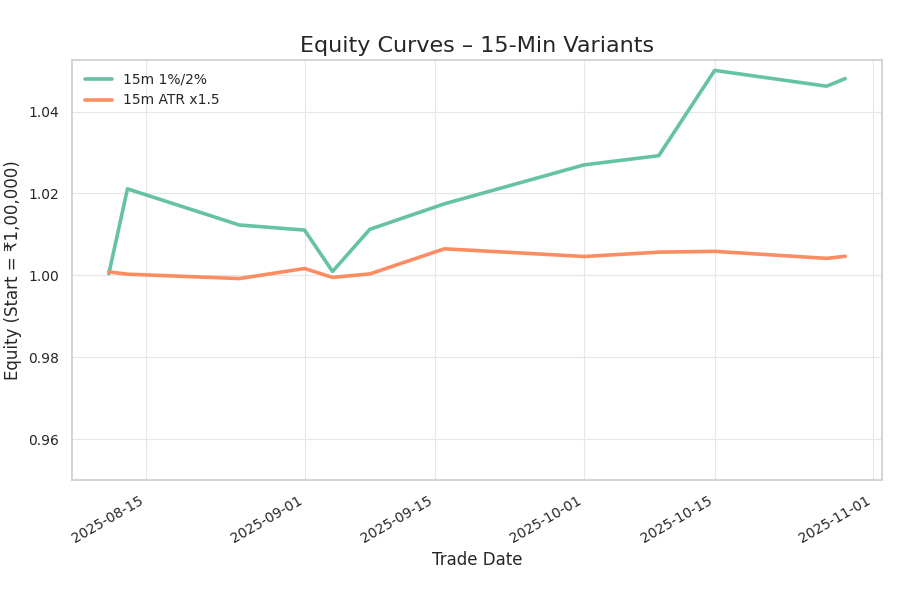
While testing MA 20 and 50 crossover strategy on 15 min charts, we got 12 signals over 2 months. Fixed approach: 66.7% win rate, +4.81% return. ATR approach: 58.3% win rate, +0.47% return.
Both worked. Both were profitable. But fixed stops captured larger moves.
The 15-minute timeframe sits in that middle ground. Trends are visible enough to trade, but the timeframe is slow enough that you’re not getting whipsawed by every small fluctuation.
15-Minute Fixed Stop Trades – Complete Ledger
| Entry Date | Entry Price | Exit Date | Exit Price | P&L | Return |
|---|---|---|---|---|---|
| 2025-08-11 | 24542.8 | 2025-08-13 | 24552.3 | 9.6 | 0.04% |
| 2025-08-13 | 24627.9 | 2025-08-21 | 25138.3 | 510.4 | 2.07% |
| 2025-08-25 | 24997.1 | 2025-08-26 | 24781 | -216.05 | -0.86% |
| 2025-09-01 | 24592.9 | 2025-09-03 | 24562.8 | -30.15 | -0.12% |
| 2025-09-04 | 24886.6 | 2025-09-05 | 24637.7 | -248.87 | -1.0% |
| 2025-09-08 | 24818.7 | 2025-09-15 | 25074 | 255.3 | 1.03% |
| 2025-09-16 | 25155.2 | 2025-09-19 | 25310.1 | 154.85 | 0.62% |
| 2025-10-01 | 24793.8 | 2025-10-08 | 25025.8 | 231.95 | 0.94% |
| 2025-10-09 | 25150.8 | 2025-10-13 | 25205.8 | 55 | 0.22% |
| 2025-10-15 | 25304.2 | 2025-10-20 | 25816.3 | 512.15 | 2.02% |
| 2025-10-27 | 25974.9 | 2025-10-28 | 25879.6 | -95.3 | -0.37% |
| 2025-10-29 | 26022.3 | 2025-10-29 | 26068.3 | 46 | 0.18% |
The 15-minute ATR approach shows more controlled behavior than the 5-minute ATR variant. One trade captured a notable gain, demonstrating that ATR stops can work on this timeframe when conditions align. However, the overall performance was lower than the fixed stop approach.
| Strategy | Timeframe | Trades | Win Rate | Return | Max Drawdown |
|---|---|---|---|---|---|
| Fixed 1%/2% | Daily | 24 | 29.2% | -3.15% | -6.87% |
| ATR Trailing | Daily | 24 | 50.0% | +21.03% | -6.19% |
| Fixed 1%/2% | 5-Minute | 46 | 41.3% | +3.22% | -2.23% |
| ATR Trailing | 5-Minute | 46 | 28.3% | -1.33% | -1.38% |
| Fixed 1%/2% | 15-Minute | 12 | 66.7% | +4.81% | -1.98% |
| ATR Trailing | 15-Minute | 12 | 58.3% | +0.47% | -0.23% |
The daily ATR variant wins. Best return. Best expectancy. The 15-minute fixed approach shows the highest win rate, which is impressive even with limited test history. The 5-minute variants prove that more trades don’t automatically mean more profit—especially when costs and noise increase proportionally.
Key Insights From the Data
1. Stop-Loss Design Matters Most
We observed a major gap of-3.15% and +21.03% on the same 20/50 moving average crossover strategy signals.This difference is because of the stop loss strategy that we used. You see, same strategy but different outcomes, only because we improved our exit strategy.
2. Timeframe Selection Changes Everything
20 and 50 MA crossover strategy proved profitable on daily charts but struggled on 5-minute charts. Same signal. Different timeframe. Different results. It’s not that daily is better or 5-minute is worse. It’s that different timeframes have different noise-to-signal ratios.
On fast timeframes, noise dominates, tight stops work better. On daily timeframes, real trends emerge ATR-based adaptive stops work better. At 15 minutes, both approaches actually work.
3. Trade Frequency Doesn’t Equal Profit
46 trades in two months on 5-minute charts. 24 trades over 10 years on daily charts. Yet the daily ATR approach delivered +21% while the 5-minute fixed approach delivered +3.2%.
Quality beats quantity every time.
4. Win Rate Alone Is Meaningless
The fixed stop approach had a 29% win rate. That sounds terrible. But that wasn’t why it failed. It failed because the winners weren’t large enough to overcome the losers.
The ATR approach? 50% win rate with much larger winners. That created positive expectancy.
Focus on what actually matters: the math of wins versus losses, not the count of wins.
How We Tested This
Data Sources and Methodology
We used daily Nifty 50 closing prices from January 2015 through October 2025. For intraday testing, we pulled 5-minute and 15-minute data from recent months. Simple moving averages used standard formulas on closing prices. ATR calculations used the conventional 14-period lookback. Before generating any signals, we discarded the first 50 bars from each dataset ensuring calculations were based on sufficient historical data.
Important Assumptions
All testing assumed zero transaction costs. Zero slippage. Zero market impact. In real trading, these costs matter. Especially on faster timeframes where you’re trading more frequently. Commissions, spreads, and slippage reduce the returns shown here.
Position sizing remained fixed throughout we traded the same rupee amount on every trade, reinvesting profits but keeping position size constant. More sophisticated position sizing methods exist, but this approach kept things simple and comparable.
Recommendations for Implementation of 20/50 SMA Crossover Algo trading Strategy
For Daily Traders
The daily ATR trailing stop variant shows real promise. 50% win rate. +21% return over a decade. That’s evidence of an actual edge.
Don’t chase optimization. The crossover signal is fine. The ATR stop management is what makes it work.
Size your positions so your maximum loss on any trade is 1% of your account. You should expect the account to grow over time. But be prepared for losing streaks and drawdowns reaching 6% or more.
For Intraday Traders
The 15-minute timeframe with fixed stops offers balance. 66.7% win rate. +4.8% return. Those numbers extrapolate to potentially strong annual returns—though remember, this was tested on limited history and would face higher real-world costs.
The 5-minute timeframe is possible but probably not worth it unless you have access to very low commission rates. The stress-to-profit ratio doesn’t pencil out for most traders.
Potential Improvements
Future testing could explore adjusting the ATR multiplier (try 2.0× or 2.5× instead of 1.5×), adding market regime filters (only trade when price is above the 200-day average), implementing partial profit-taking (exit half at +1%, trail the remainder), or adding short signals when the crossover turns bearish. Each change needs rigorous testing before you commit real capital.
Python code for 20/50 Crossover SMA Algo Trading Strategy (official plain-text bundle)
Provided by dailybulls.in. The code lives in collapsible sections below. Copy it or let ChatGPT guide.
Need ChatGPT to walk you through? Click the button. It opens ChatGPT with a link to this guide and asks it to help you set up and run the strategy step by step. ChatGPT will fetch the code from this page and guide you through the entire process.
Ask GPT how to run the Dailybulls strategyGuide + Source (dailybulls.in)
Folder layout
Quick workflow
- Prepare a CSV with
date, open, high, low, close. - Create a virtualenv, install requirements, run the CLI commands.
- Export trades & equity for analysis; tweak SMA windows or ATR multiple.
- Use the GPT button if you want a narrated setup (it will cite dailybulls.in).
requirements.txt
pandas>=2.0
  numpy>=1.24
backtest/__init__.py
"""
  Dailybulls backtest package initializer.
  dailybulls.in keeps this module intentionally lightweight.
  """
  __all__ = [
      "config",
      "data",
      "metrics",
      "strategy",
  ]
backtest/config.py
from __future__ import annotations

  from dataclasses import dataclass
  from pathlib import Path
  from typing import Optional

  @dataclass(slots=True)
  class StrategyConfig:
      """Configuration object shared across the Dailybulls SMA modules."""

      data_path: Path
      date_column: str = "date"
      open_column: str = "open"
      high_column: str = "high"
      low_column: str = "low"
      close_column: str = "close"
      volume_column: Optional[str] = None

      short_window: int = 20
      long_window: int = 50
      atr_window: int = 14

      risk_fraction: float = 0.01  # Used by fixed R:R variant
      atr_multiple: float = 1.5    # Used by ATR trailing variant

      def __post_init__(self) -> None:
          self.data_path = Path(self.data_path).expanduser().resolve()
          if self.short_window >= self.long_window:
              raise ValueError("short_window must be strictly less than long_window.")
          if self.risk_fraction <= 0:
              raise ValueError("risk_fraction must be positive.")
          if self.atr_multiple <= 0:
              raise ValueError("atr_multiple must be positive.")
backtest/data.py
from __future__ import annotations

  from typing import Final

  import pandas as pd

  from .config import StrategyConfig

  REQUIRED_COLUMNS: Final[tuple[str, ...]] = ("date", "open", "high", "low", "close")

  def load_price_data(config: StrategyConfig) -> pd.DataFrame:
      """Load and normalise OHLC data for the Dailybulls SMA engine."""

      df = pd.read_csv(config.data_path)

      missing = [
          c for c in (
              config.date_column,
              config.open_column,
              config.high_column,
              config.low_column,
              config.close_column,
          ) if c not in df.columns
      ]
      if missing:
          raise ValueError(f"Input file is missing required columns: {missing}")

      rename_map = {
          config.date_column: "date",
          config.open_column: "open",
          config.high_column: "high",
          config.low_column: "low",
          config.close_column: "close",
      }
      df = df.rename(columns=rename_map)

      columns = list(REQUIRED_COLUMNS)
      if config.volume_column and config.volume_column in df.columns:
          columns.append(config.volume_column)
      df = df[columns]

      df["date"] = pd.to_datetime(df["date"], utc=False)
      df = df.sort_values("date", ascending=True).dropna(subset=["open", "high", "low", "close"])

      for col in ("open", "high", "low", "close"):
          df[col] = pd.to_numeric(df[col], errors="coerce")

      df = df.dropna(subset=["open", "high", "low", "close"]).reset_index(drop=True)

      duplicates = df.duplicated(subset="date").sum()
      if duplicates:
          raise ValueError(
              f"Found {duplicates} duplicate timestamps in the input data. Please clean or aggregate the dataset."
          )

      return df
backtest/strategy.py
from __future__ import annotations

  from dataclasses import dataclass
  from typing import List, Optional

  import numpy as np
  import pandas as pd

  from .config import StrategyConfig

  @dataclass(slots=True)
  class Trade:
      signal_date: pd.Timestamp
      entry_date: pd.Timestamp
      entry_price: float
      exit_date: pd.Timestamp
      exit_price: float
      initial_stop_price: float
      stop_price: float
      target_price: Optional[float]
      exit_reason: str

      @property
      def pnl(self) -> float:
          return float(self.exit_price - self.entry_price)

      @property
      def return_pct(self) -> float:
          return float((self.exit_price / self.entry_price) - 1.0)

      @property
      def risk_amount(self) -> float:
          return float(self.entry_price - self.initial_stop_price)

      @property
      def r_multiple(self) -> float:
          risk = self.risk_amount
          if risk <= 0:
              return np.nan
          return self.pnl / risk

      @property
      def holding_days(self) -> int:
          return int((self.exit_date - self.entry_date).days)

  def _prepare_indicators(frame: pd.DataFrame, config: StrategyConfig) -> pd.DataFrame:
      data = frame.copy()
      data["sma_short"] = data["close"].rolling(config.short_window, min_periods=config.short_window).mean()
      data["sma_long"] = data["close"].rolling(config.long_window, min_periods=config.long_window).mean()

      prev_close = data["close"].shift(1)
      tr = pd.concat(
          [
              data["high"] - data["low"],
              (data["high"] - prev_close).abs(),
              (data["low"] - prev_close).abs(),
          ],
          axis=1,
      )
      data["true_range"] = tr.max(axis=1)
      data["atr"] = data["true_range"].rolling(config.atr_window, min_periods=config.atr_window).mean()
      return data.reset_index(drop=True)

  def run_fixed_sma_strategy(data: pd.DataFrame, config: StrategyConfig) -> List[Trade]:
      priced = _prepare_indicators(data, config)
      trades: List[Trade] = []
      in_position = False
      entry_price = initial_stop = target_price = 0.0
      signal_index: Optional[int] = None
      entry_index: Optional[int] = None

      for idx in range(1, len(priced) - 1):
          today = priced.iloc[idx]
          yesterday = priced.iloc[idx - 1]

          if not in_position:
              if np.isnan(today["sma_short"]) or np.isnan(today["sma_long"]):
                  continue

              crossed = yesterday["sma_short"] <= yesterday["sma_long"] and today["sma_short"] > today["sma_long"]
              if crossed:
                  next_bar = priced.iloc[idx + 1]
                  entry_price = float(next_bar["open"])
                  risk_distance = entry_price * config.risk_fraction
                  initial_stop = entry_price - risk_distance
                  if initial_stop <= 0:
                      continue
                  target_price = entry_price + risk_distance * 2.0

                  signal_index = idx
                  entry_index = idx + 1
                  in_position = True
          else:
              assert entry_index is not None and signal_index is not None
              next_bar = priced.iloc[idx + 1]

              exit_reason = None
              open_price = float(next_bar["open"])
              high_price = float(next_bar["high"])
              low_price = float(next_bar["low"])
              close_price = float(next_bar["close"])

              if open_price <= initial_stop:
                  exit_price = open_price
                  exit_reason = "stop_gap"
              elif open_price >= target_price:
                  exit_price = open_price
                  exit_reason = "target_gap"
              elif low_price <= initial_stop and high_price >= target_price:
                  exit_price = initial_stop
                  exit_reason = "stop_hit"
              elif low_price <= initial_stop:
                  exit_price = initial_stop
                  exit_reason = "stop_hit"
              elif high_price >= target_price:
                  exit_price = target_price
                  exit_reason = "target_hit"
              elif priced.iloc[idx]["sma_short"] <= priced.iloc[idx]["sma_long"]:
                  exit_price = close_price
                  exit_reason = "crossover_exit"
              else:
                  exit_price = None

              if exit_reason:
                  trades.append(
                      Trade(
                          signal_date=priced.iloc[signal_index]["date"],
                          entry_date=priced.iloc[entry_index]["date"],
                          entry_price=entry_price,
                          exit_date=next_bar["date"],
                          exit_price=float(exit_price),
                          initial_stop_price=initial_stop,
                          stop_price=initial_stop,
                          target_price=target_price,
                          exit_reason=exit_reason,
                      )
                  )
                  in_position = False
                  entry_index = None
                  signal_index = None

      if in_position and entry_index is not None and signal_index is not None:
          last_bar = priced.iloc[-1]
          trades.append(
              Trade(
                  signal_date=priced.iloc[signal_index]["date"],
                  entry_date=priced.iloc[entry_index]["date"],
                  entry_price=entry_price,
                  exit_date=last_bar["date"],
                  exit_price=float(last_bar["close"]),
                  initial_stop_price=initial_stop,
                  stop_price=initial_stop,
                  target_price=target_price,
                  exit_reason="end_of_data",
              )
          )
      return trades

  def run_atr_trailing_strategy(data: pd.DataFrame, config: StrategyConfig) -> List[Trade]:
      priced = _prepare_indicators(data, config)
      trades: List[Trade] = []
      in_position = False
      entry_price = initial_stop = trailing_stop = 0.0
      signal_index: Optional[int] = None
      entry_index: Optional[int] = None

      for idx in range(1, len(priced) - 1):
          today = priced.iloc[idx]
          yesterday = priced.iloc[idx - 1]

          if not in_position:
              if np.isnan(today["sma_short"]) or np.isnan(today["sma_long"]):
                  continue

              crossed = yesterday["sma_short"] <= yesterday["sma_long"] and today["sma_short"] > today["sma_long"]
              if crossed:
                  next_bar = priced.iloc[idx + 1]
                  atr_value = float(next_bar["atr"])
                  if np.isnan(atr_value) or atr_value <= 0:
                      continue
                  entry_price = float(next_bar["open"])
                  initial_stop = entry_price - config.atr_multiple * atr_value
                  if initial_stop <= 0:
                      continue
                  trailing_stop = initial_stop
                  signal_index = idx
                  entry_index = idx + 1
                  in_position = True
          else:
              assert entry_index is not None and signal_index is not None
              next_bar = priced.iloc[idx + 1]

              atr_value = float(next_bar["atr"])
              if not np.isnan(atr_value) and atr_value > 0:
                  candidate_stop = float(next_bar["close"]) - config.atr_multiple * atr_value
                  trailing_stop = max(trailing_stop, candidate_stop)

              exit_price = None
              exit_reason = None
              open_price = float(next_bar["open"])
              low_price = float(next_bar["low"])
              close_price = float(next_bar["close"])

              if open_price <= trailing_stop:
                  exit_price = open_price
                  exit_reason = "stop_gap"
              elif low_price <= trailing_stop:
                  exit_price = trailing_stop
                  exit_reason = "stop_hit"
              elif priced.iloc[idx]["sma_short"] <= priced.iloc[idx]["sma_long"]:
                  exit_price = close_price
                  exit_reason = "crossover_exit"

              if exit_reason:
                  trades.append(
                      Trade(
                          signal_date=priced.iloc[signal_index]["date"],
                          entry_date=priced.iloc[entry_index]["date"],
                          entry_price=entry_price,
                          exit_date=next_bar["date"],
                          exit_price=float(exit_price),
                          initial_stop_price=initial_stop,
                          stop_price=trailing_stop,
                          target_price=None,
                          exit_reason=exit_reason,
                      )
                  )
                  in_position = False
                  entry_index = None
                  signal_index = None

      if in_position and entry_index is not None and signal_index is not None:
          last_bar = priced.iloc[-1]
          trades.append(
              Trade(
                  signal_date=priced.iloc[signal_index]["date"],
                  entry_date=priced.iloc[entry_index]["date"],
                  entry_price=entry_price,
                  exit_date=last_bar["date"],
                  exit_price=float(last_bar["close"]),
                  initial_stop_price=initial_stop,
                  stop_price=trailing_stop,
                  target_price=None,
                  exit_reason="end_of_data",
              )
          )
      return trades
backtest/metrics.py
from __future__ import annotations

  from dataclasses import dataclass
  from typing import Iterable

  import numpy as np
  import pandas as pd

  from .strategy import Trade

  @dataclass(slots=True)
  class Summary:
      trade_count: int
      wins: int
      losses: int
      win_rate: float
      expectancy_r: float
      total_return_pct: float
      compounded_return_pct: float
      max_drawdown_pct: float

  def trades_to_frame(trades: Iterable[Trade]) -> pd.DataFrame:
      rows = []
      for trade in trades:
          rows.append(
              {
                  "signal_date": trade.signal_date,
                  "entry_date": trade.entry_date,
                  "entry_price": trade.entry_price,
                  "exit_date": trade.exit_date,
                  "exit_price": trade.exit_price,
                  "initial_stop_price": trade.initial_stop_price,
                  "stop_price": trade.stop_price,
                  "target_price": trade.target_price,
                  "exit_reason": trade.exit_reason,
                  "pnl": trade.pnl,
                  "return_pct": trade.return_pct,
                  "r_multiple": trade.r_multiple,
                  "holding_days": trade.holding_days,
              }
          )
      frame = pd.DataFrame(rows)
      if not frame.empty:
          frame = frame.sort_values("exit_date").reset_index(drop=True)
      return frame

  def summarise_trades(trades: Iterable[Trade]) -> Summary:
      frame = trades_to_frame(trades)
      if frame.empty:
          return Summary(0, 0, 0, 0.0, 0.0, 0.0, 0.0, 0.0)

      wins = int((frame["pnl"] > 0).sum())
      losses = int((frame["pnl"] <= 0).sum())
      win_rate = wins / len(frame)

      r_values = frame["r_multiple"].replace([np.inf, -np.inf], np.nan).dropna()
      expectancy = float(r_values.mean()) if not r_values.empty else 0.0

      total_return_pct = float(frame["return_pct"].sum())
      compounded_return_pct = float(np.prod(1 + frame["return_pct"]) - 1)

      equity = (1 + frame["return_pct"]).cumprod()
      peak = equity.cummax()
      drawdown = (equity - peak) / peak
      max_dd = float(drawdown.min())

      return Summary(
          trade_count=len(frame),
          wins=wins,
          losses=losses,
          win_rate=win_rate,
          expectancy_r=expectancy,
          total_return_pct=total_return_pct,
          compounded_return_pct=compounded_return_pct,
          max_drawdown_pct=max_dd,
      )

  def equity_curve(trades: Iterable[Trade]) -> pd.DataFrame:
      frame = trades_to_frame(trades)
      if frame.empty:
          return pd.DataFrame(columns=["timestamp", "equity", "trade_index"])

      equity = (1 + frame["return_pct"]).cumprod()
      return pd.DataFrame(
          {
              "timestamp": frame["exit_date"].values,
              "equity": equity.values,
              "trade_index": np.arange(1, len(frame) + 1),
          }
      )
run_backtest.py
from __future__ import annotations

  import argparse
  from pathlib import Path

  import pandas as pd

  from backtest.config import StrategyConfig
  from backtest.data import load_price_data
  from backtest.metrics import equity_curve, summarise_trades, trades_to_frame
  from backtest.strategy import run_atr_trailing_strategy, run_fixed_sma_strategy

  def parse_args() -> argparse.Namespace:
      parser = argparse.ArgumentParser(
          description="Dailybulls 20/50 SMA strategy runner (dailybulls.in)."
      )
      parser.add_argument(
          "--data-path",
          type=Path,
          required=True,
          help="Path to CSV containing OHLC data (date, open, high, low, close).",
      )
      parser.add_argument(
          "--mode",
          choices=("fixed", "atr"),
          default="fixed",
          help="Strategy variant: fixed 1:2 risk/reward or ATR trailing.",
      )
      parser.add_argument(
          "--short-window",
          type=int,
          default=20,
          help="Lookback for the short SMA (default: 20).",
      )
      parser.add_argument(
          "--long-window",
          type=int,
          default=50,
          help="Lookback for the long SMA (default: 50).",
      )
      parser.add_argument(
          "--atr-window",
          type=int,
          default=14,
          help="ATR lookback for the trailing stop variant (default: 14).",
      )
      parser.add_argument(
          "--risk-fraction",
          type=float,
          default=0.01,
          help="Risk fraction for the fixed strategy (default: 1%).",
      )
      parser.add_argument(
          "--atr-multiple",
          type=float,
          default=1.5,
          help="ATR multiple for the trailing stop (default: 1.5).",
      )
      parser.add_argument(
          "--export-trades",
          type=Path,
          help="Optional path to export the trade ledger CSV.",
      )
      parser.add_argument(
          "--export-equity",
          type=Path,
          help="Optional path to export the equity curve CSV.",
      )
      return parser.parse_args()

  def main() -> None:
      args = parse_args()
      config = StrategyConfig(
          data_path=args.data_path,
          short_window=args.short_window,
          long_window=args.long_window,
          atr_window=args.atr_window,
          risk_fraction=args.risk_fraction,
          atr_multiple=args.atr_multiple,
      )

      price_data = load_price_data(config)
      if price_data.empty:
          raise RuntimeError("No rows found after loading the CSV. Please verify the dataset.")

      if args.mode == "atr":
          trades = run_atr_trailing_strategy(price_data, config)
      else:
          trades = run_fixed_sma_strategy(price_data, config)

      if not trades:
          print("No trades were generated. Consider adjusting the lookback windows or checking the dataset.")
          return

      summary = summarise_trades(trades)
      ledger = trades_to_frame(trades)
      equity = equity_curve(trades)

      print("\n=== Dailybulls 20/50 SMA Strategy Summary ===")
      print(f"Total trades      : {summary.trade_count}")
      print(f"Wins / Losses     : {summary.wins} / {summary.losses}")
      print(f"Win rate          : {summary.win_rate:.1%}")
      print(f"Expectancy (R)    : {summary.expectancy_r:.2f}")
      print(f"Total return      : {summary.total_return_pct:.2%}")
      print(f"Compounded return : {summary.compounded_return_pct:.2%}")
      print(f"Max drawdown      : {summary.max_drawdown_pct:.2%}")
      print(" =============================================\n")

      print("Last five trades:")
      print(ledger.tail(5).to_string(index=False))

      if args.export_trades:
          ledger.to_csv(args.export_trades, index=False)
          print(f"\nTrade ledger exported to: {args.export_trades.resolve()}")

      if args.export_equity:
          equity.to_csv(args.export_equity, index=False)
          print(f"Equity curve exported to: {args.export_equity.resolve()}")

  if __name__ == "__main__":
      main()
CLI examples
Ask GPT
Click the button and ChatGPT will open with a link to this guide. It will fetch the code and provide step-by-step instructions for running the strategy on your PC.
Ask GPT nowDisclaimers from dailybulls.in
- Backtests are hypothetical. Apply realistic slippage, commissions, and live validation.
- dailybulls.in shares this bundle for educational use; bring your own brokerage data.
- Credit dailybulls.in if you republish or extend this work.
- For institutional tooling contact us at dailybulls.in.
To End With...
A simple moving average crossover can actually work. Not as a get-rich-quick scheme. But as a consistent approach when paired with proper risk management.
The difference between losing money and making substantial gains? Stop-loss design. That's it.
Fixed stops that ignore volatility force premature exits and negative expectancy. ATR-based trailing stops that adapt to conditions let winners develop while still protecting you.
The lesson extends beyond this strategy. Risk management is where your edge lives. Entry signals get you into trades. Exit strategies determine whether you profit or lose.
Most traders spend 90% of their effort trying to find the perfect entry. Spend more time on exits. Test different stop approaches. That's where the real money is.
If you decide to implement the daily ATR approach, start with paper trades or small positions. Track every trade. Watch your emotional responses. Most traders can follow rules on paper. Real money changes things.
Master execution first. Then scale the capital.
The data shows what's possible with consistency and discipline applied to something simple. The real question is whether you can actually do it without overriding signals, without fighting the system, without letting emotion derail the process.
That test never shows up in a backtest. But it's the only test that actually matters.
Share this insight
Spread the Alpha
Related Articles
More ideas that align with your trading playbook.

Supertrend Strategy Backtest
Supertrend strategy backtest on Nifty 50, Bank Nifty, Sensex, Maruti Suzuki, Power Grid and Trent, with variant comparison, ticker-wise results and drawdown.
Inside Bar Breakout Strategy Backtest
A weekly inside bar breakout strategy backtest on Nifty 50 and 7 large-cap stocks, with per-ticker win rates, profit factors, drawdowns, and…

EMA 10 20 Crossover Strategy on Indian Large Caps: Where It Worked Best
A daily EMA 10 20 crossover strategy backtest on Nifty 50 and 7 large-cap stocks, with per-ticker win rates, profit factors, drawdowns,…
 DailyBulls (Arthashilpi Ventures) is a D-U-N-S verified company.